How to use a VLOOKUP in Google Sheets

Google Sheets has several built-in functions to help you perform calculations and find data in your spreadsheets. One essential function, especially if you work with large, complex spreadsheets, is the VLOOKUP function.

Google Sheets VLOOKUP saves you time and effort when locating specific data points or cross-referencing data in spreadsheets. 

Learn how it works below. 

<a href="#vlookup-intro" class="anchor-link">What is the Google Sheets VLOOKUP function?</a>
<a href="#vlookup-tips" class="anchor-link">5 important things to know about VLOOKUP in Google Sheets</a>
<a href="#create-vlookup" class="anchor-link">How to create your own Google Sheets VLOOKUP</a>
<a href="#vlookup-multiple" class="anchor-link">Copy a VLOOKUP formula across cells and compile data from multiple sheets</a>
<a href="#vlookup-business" class="anchor-link">Real-world business applications of the VLOOKUP function</a>

<div class="anchor-wrapper"><div id="vlookup-intro" class="anchor-target"></div></div>

What is the Google Sheets VLOOKUP function? 

VLOOKUP is a Google Sheets function that stands for “Vertical lookup.” This tool allows you to search for a specific entry in a column of data to find corresponding data from that row if there’s a match.  

Think of it like looking for your grade on a posted list (back when that was the way people checked their grades, anyway). The professor puts up a paper with two columns: student names and grades. You scan the first column for your name, locate it, then move straight into the second column to find your grade. The VLOOKUP function does that manual searching for you and automatically returns the information you need, as long as there’s a match for your search. 

The function formula is: =VLOOKUP(search_key, range, index, [is_sorted])

It includes the following four parts:

• Search_key: The identifying data point you’re searching for (ie your name).
• Range: The cells that contain the columns from which you want to retrieve data - this is where you’re telling the formula to search for your answer.
• Index: The column with the return value (ie your grade).
• Is_sorted: A true or false value where FALSE means the exact match and TRUE means the nearest match (99% of the time, FALSE is the preferred setting.)

VLOOKUPs can also be used to find data points that may be spread across various sheets so you can compile your data. For SQL users, this is equivalent to a Left Outer Join. 

Keep reading for examples and step-by-step instructions.

<div class="anchor-wrapper"><div id="vlookup-tips" class="anchor-target"></div></div>

5 important things to know about VLOOKUP in Google Sheets

Although the VLOOKUP formula seems simple enough at face value, there are a couple tricks to making sure you’re getting the correct data in your search results. 

1. Lookup values must be in the first column of the range

With VLOOKUP, your lookup value must be in the first (farthest left) column of the range you're working with. If the value is in a column to the right of the information you're looking for, the function won't work.

2. VLOOKUP is not case sensitive in Google Sheets

The VLOOKUP function in Google Sheets does not differentiate between uppercase and lowercase letters. For a case-sensitive lookup, you would need to use other functions or scripting.

3. VLOOKUP returns the first match

VLOOKUP stops at the first match it finds. If there are multiple matches in your range, the function will only return the value associated with the first one it comes across.

4. Use absolute cell references to copy across multiple cells

In Google Sheets, you'll want to use absolute cell references for the range when applying the VLOOKUP function and copying it down or across other cells. For instance, instead of A1:D100, use $A$1:$D$100. Without these, when you drag the formula down or across, Google Sheets will automatically adjust the cell references, leading to incorrect results.

5. Approximate and exact matches

By default, VLOOKUP in Google Sheets performs an approximate match, which requires that your first column be sorted in ascending order. If you want to find an exact match, you need to set the optional fourth argument to FALSE. Without this, VLOOKUP might return unexpected results if an exact match isn't found.

<div class="anchor-wrapper"><div id="create-vlookup" class="anchor-target"></div></div>

How to create your own Google Sheets VLOOKUP function

To create your own VLOOKUP function, open up a Google Sheets spreadsheet. Ensure all your data is organized in clearly labeled columns and you know what you’re looking for. Then, put the function to work. Here’s how:

1. Set up your spreadsheet.

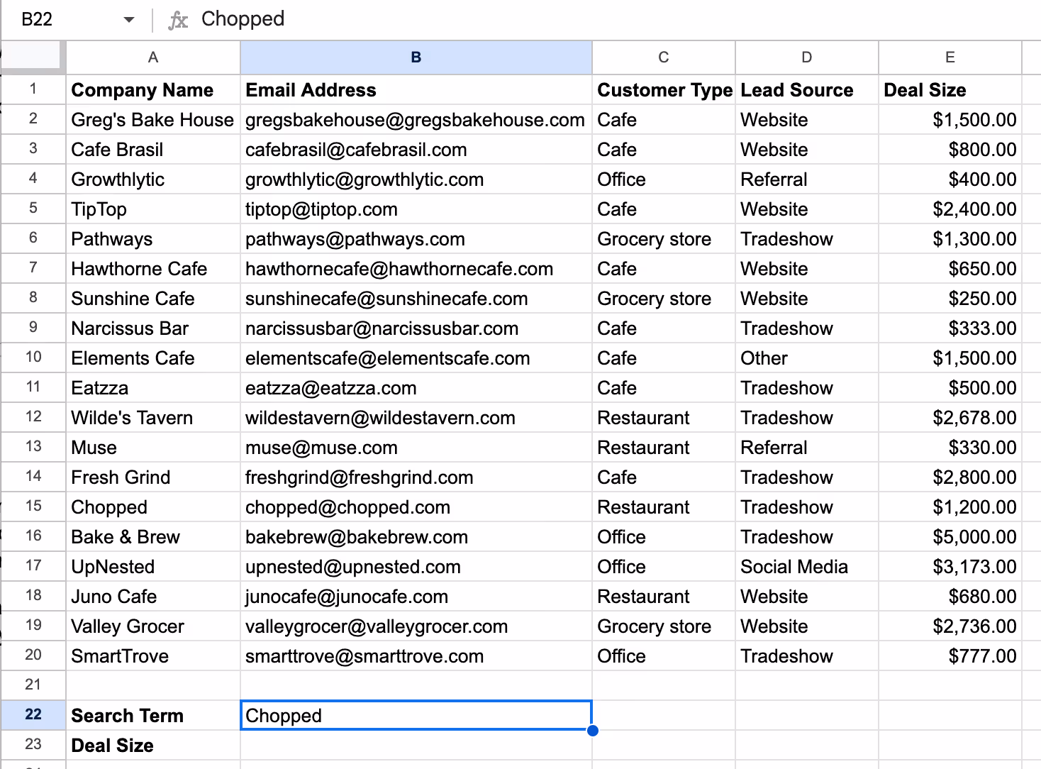
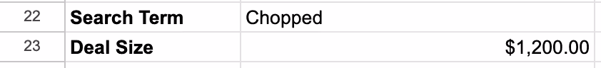
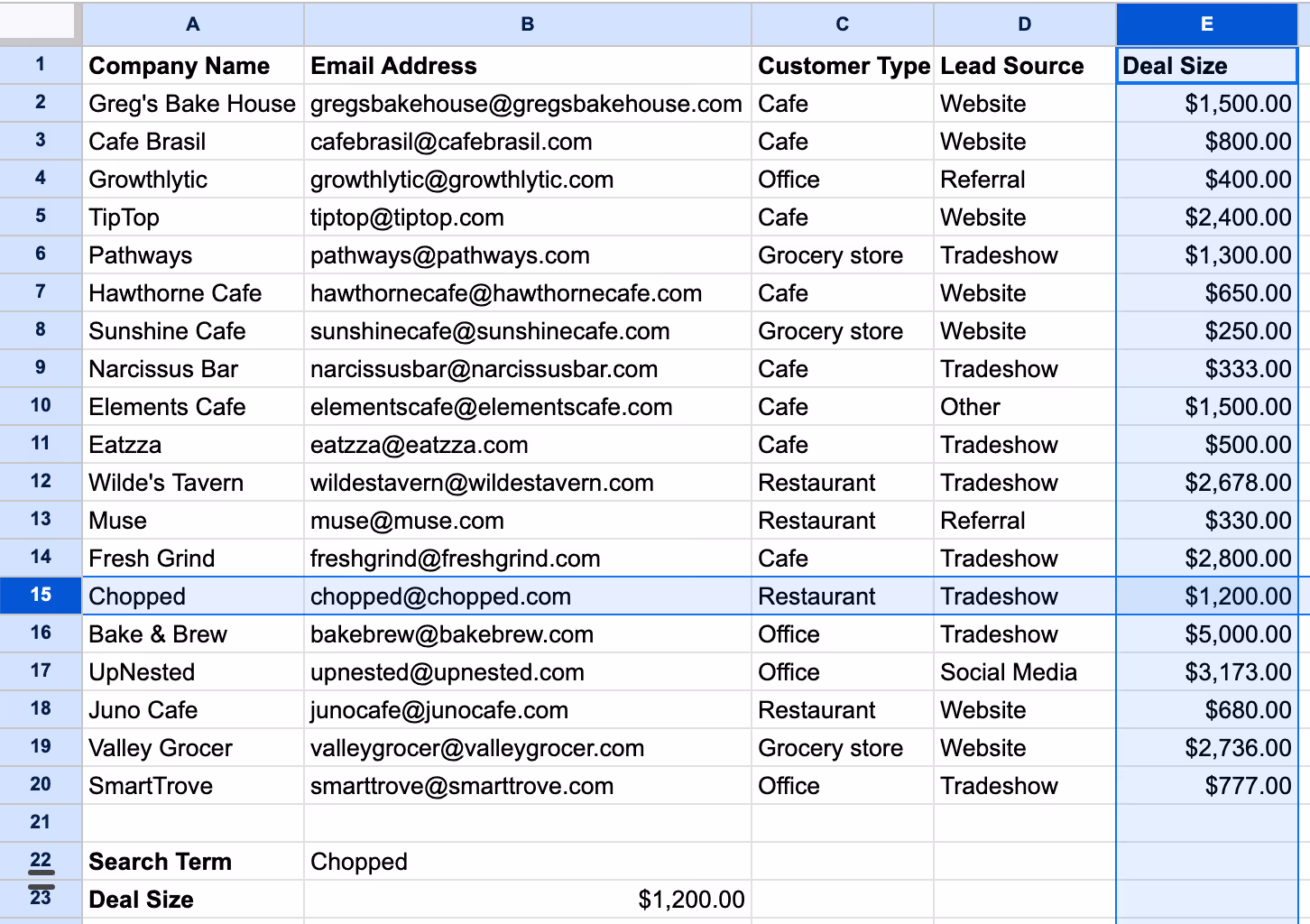
Stay organized by typing two labels below or to the side of your data: Search term and the label for the return value you’re looking for (Deal Size in this example). Type (or copy) your search term into the box next to the label. In this example, we’re looking for data related to the company Chopped in our list, so we use that as the search term. Make sure your search term is identical to how it appears in your data set. 

‍

2. Add a VLOOKUP formula

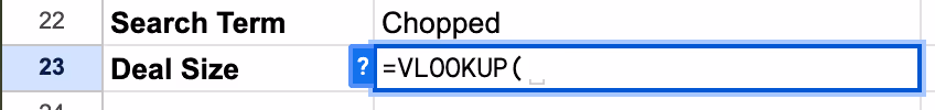
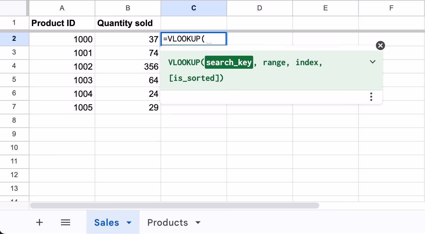
In the next box, start typing your formula with an equal sign followed by VLOOKUP and an open parenthesis.

3. Tell it what to look for

The search_key portion of the formula tells it what piece of data you want to find a result for.

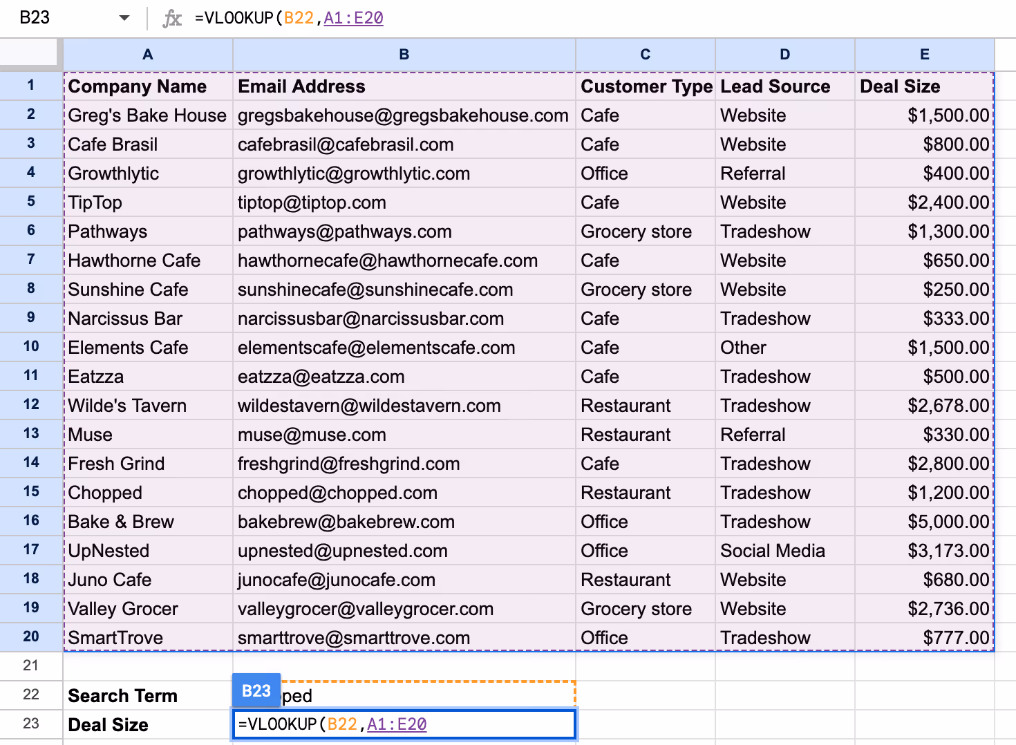
To select the search_key, click the cell containing your search term. In our example, this is the cell containing “Chopped”. When you type a different value into the search_key cell, the VLOOKUP will search for results corresponding with that value. Google Sheets will highlight the box you selected by outlining it with a colorful dotted line and the cell number will automatically fill in your formula. Alternatively, you can type the cell number - for example: “B22”.

Type a comma to separate the values in the formula.

4. Tell it where to look

The range tells your formula where to look by specifying what data to consider in the search. Enter the range by clicking and dragging on the spreadsheet to select all the data you want to include in your search. In this case, that’s all five columns of data in the spreadsheet. Add a comma to move to the next input.

5. Enter your index

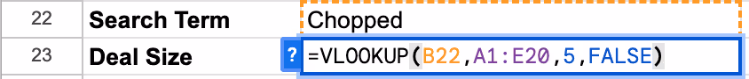
The index tells your VLOOKUP which column it should pull the answers from. Type in the number (in digit form) of the column you want to retrieve data from, followed by a comma. Since the “Deal Size” information is in the fifth column from the left, we’ll type in the digit “5.” Do not highlight the column or enter the column name here—the formula won’t recognize those forms.

Type another comma for your final formula value.

6. Exact search term vs. approximate matching

For an exact match for your search term, enter FALSE or 0. Type in TRUE or 1 for approximate matching, but that’s generally not necessary. Finish out the formula with a closing parenthesis.

7. Complete your formula

Press enter to see the results of your search. In this example, the function returned the result of a $1,200 estimated deal size for Chopped.

8. Check your answers

The first few times you use the function, you may want to check your results manually to ensure you’re entering everything correctly. 

For this example, a manual search shows that the function returned the right deal size for Chopped. 

<div class="anchor-wrapper"><div id="vlookup-multiple" class="anchor-target"></div></div>

Copy a VLOOKUP formula across cells and compile data from multiple sheets

Once you know how to create a VLOOKUP, it can be a powerful tool for spreadsheet users. A common problem that it helps solve is to compile or cross reference data in multiple spreadsheets. 

For example, suppose a sales manager has two spreadsheets. Spreadsheet A contains sales data with a list of product IDs and the quantities sold, while Spreadsheet B has detailed information about each product, including the product ID, product name, and price.

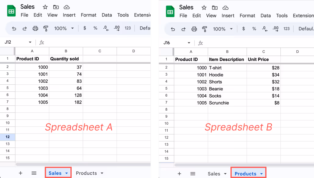
In order to calculate the total revenue from each product sold in Spreadsheet A, they need to know the price of each product. Instead of manually looking up and copying the price for each product from Spreadsheet B, they can use VLOOKUP to fill in the data in Spreadsheet A.

VLOOKUP in multiple spreadsheet cells

To achieve this, the VLOOKUP function can be copied across multiple cells of Spreadsheet A and use a range in Spreadsheet B. 

Here’s how: 

1. Prepare your spreadsheet

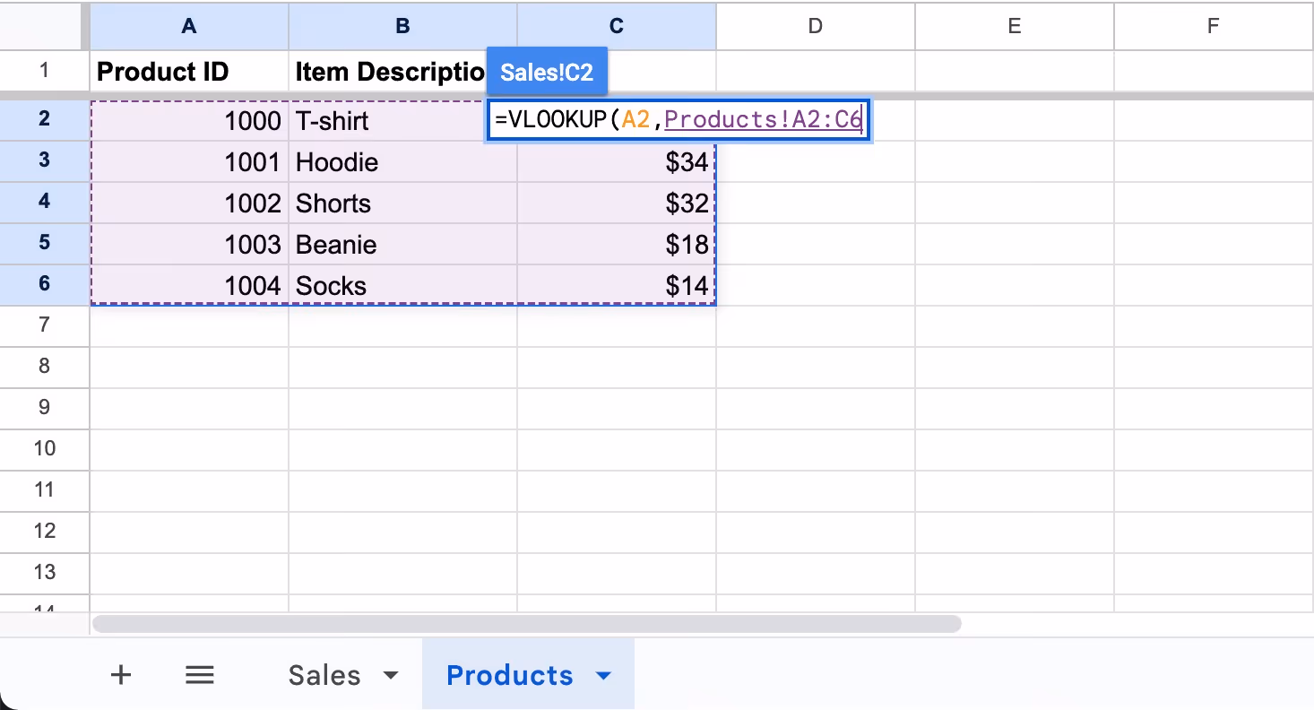
Start with a single spreadsheet document with all of your data in columns or separate sheets (tabs) of the same document, like the example above. 

Make sure the column with the search_key is to the left of the column that contains your index (search results).

2. Create a VLOOKUP formula

Write the VLOOKUP formula in a cell of Spreadsheet A.

3. Add a search-key

Add the search_key, which would be the product ID or A2.

4. Select your range.

To reference a range in another sheet, simply open the other sheet and drag your cursor over the range you want to select. You’ll see the VLOOKUP formula carries over so you can keep working on it in this sheet. You can also type the name of the Sheet in single apostrophes before the range selection. For example: ‘Products’!A2:C6.

5. Enter your index‍

Type the number of the column where you’ll find the search results.

6. Exact match?

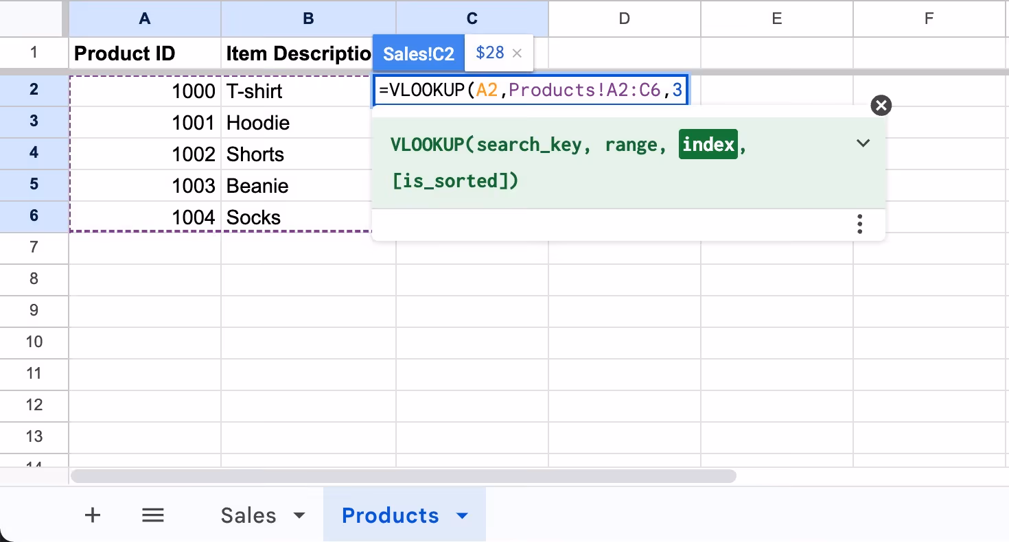
In most cases, you’ll want an exact match, so your is_sorted should be FALSE. 

Add a closed parenthesis.

7. Check results

Enter your formula, and check that you’re getting the correct result in Spreadsheet A.

8. Copy your VLOOKUP across multiple cells

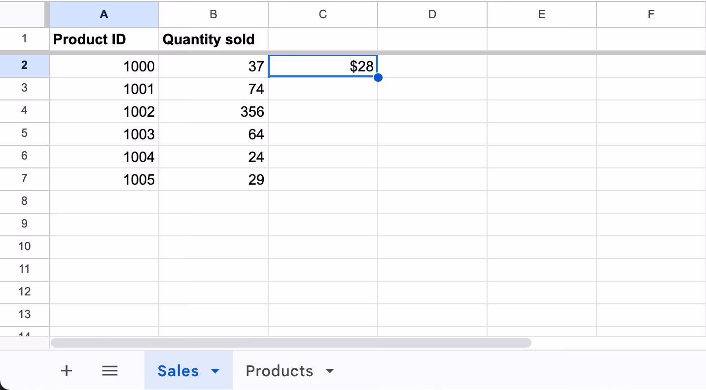
To copy the formula across multiple cells, click the blue dot in the bottom-right corner of the cell containing your VLOOKUP formula and drag it downwards to every cell where you want to return a result.

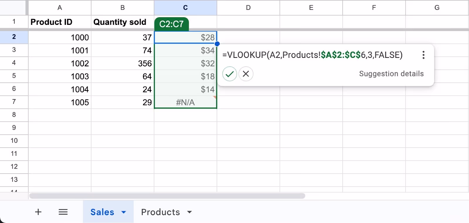
The function will be replicated in each of the selected cells, updating relative cell references according to their position. This feature allows you to perform the same lookup operation on an entire column or row of data, saving considerable time and effort if you're working with large datasets.

Keep in mind, if you need to keep certain cell references static (not changing when the formula is copied to other cells), you should use absolute references by adding a dollar sign ($) before the column letter and/or row number in the reference (e.g., $A$1). This will prevent those references from changing as you copy the formula to other cells.

<div class="anchor-wrapper"><div id="vlookup-business" class="anchor-target"></div></div>

Real-world business applications of the VLOOKUP function

At face value, the VLOOKUP function may seem like an abstract concept. To understand how powerful this can be, explore how you can actually use the Google Sheets VLOOKUP function in your workflow. 

Anytime you have a large, complex spreadsheet and need to find specific data points, VLOOKUP is helpful. Using the function saves you the time and effort of manually digging through all your data to find the necessary information. 

Finding details about sales leads

Many small to medium-sized businesses track their sales leads in lengthy spreadsheets. They record details like the lead’s name, contact information, lead source, budget or estimated deal size, and the products/services the lead is interested in. These spreadsheets quickly become unmanageable as the business adds more and more leads.

Say, for example, you have a sales lead spreadsheet with 100 leads and 16 columns containing details about each lead. That’s over 1,500 data points! If you need facts about an individual sales lead, it’s like looking for a needle in a haystack. 

Instead of scanning your list of leads for the company you’re looking for and moving horizontally to the relevant column, use VLOOKUP. The function will return the information you need about the lead without manual searching. 

Locating information about potential hires

Another scenario when VLOOKUP is useful is when you have a spreadsheet full of potential hires. As people apply for jobs at your company, you may record details such as their names, emails or phone numbers, the positions they’re applying for, and the people who referred them (if applicable). 

When it’s time to interview one of these candidates, you probably want to have information like who referred them on hand. The VLOOKUP function retrieves this information from your potential hires spreadsheet without hassle. 

Looking up customer data

You may also have spreadsheets full of sales and customer data to track order numbers, order values, customer names, and other details. These spreadsheets get so large and complex that there’s simply no good way to look through them manually. Luckily, the VLOOKUP function means you don’t have to. 

Use VLOOKUP to see how much a specific customer has spent on your products or services, for example. Or, find an order number corresponding to that customer. VLOOKUP finds and returns those details so you don’t have to hunt them down in dense sales spreadsheets. 

Inventory management

A warehouse might keep one spreadsheet with inventory details like SKU or barcode and another with corresponding item details such as cost, supplier, or item descriptions. 

By using VLOOKUP, the warehouse could quickly access specific item details just by inputting the SKU or barcode. This simplifies the process of tracking inventory and can help quickly identify information like the cost of items or which supplier they come from.

Find and compile data faster in Google Sheets

The VLOOKUP function is Google Sheets is especially valuable when handling large volumes of data or managing datasets that are split across multiple sources, as it allows for rapid and accurate data matching. This function not only saves time but also reduces the likelihood of errors that could occur from manual data lookups.

A solid understanding of VLOOKUP can greatly enhance your data handling capabilities, making data analysis and reporting processes more efficient and reliable. Instead of spending time manually digging through spreadsheets, use the VLOOKUP function to pinpoint the data you need in just a few clicks.